books
Functions
In the context of programming, a function is a named sequence of statements that performs a computation. When you define a function, you specify the name and the sequence of statements. Later, you can “call” the function by name.
3.1 Function calls
We have already seen one example of a function call:
>>> type(42)
<class 'int'>
The name of the function is type. The expression in parentheses is called the argument of the function. The result, for this function, is the type of the argument.
It is common to say that a function “takes” an argument and “returns” a result. The result is also called the return value.
Python provides functions that convert values from one type to another. The int function takes any value and converts it to an integer, if it can, or complains otherwise:
>>> int('32')
32
>>> int('Hello')
ValueError: invalid literal for int(): Hello
int can convert floating-point values to integers, but it doesn’t round off; it chops off the fraction part:
>>> int(3.99999)
3
>>> int(-2.3)
-2
float converts integers and strings to floating-point numbers:
>>> float(32)
32.0
>>> float('3.14159')
3.14159
Finally, str converts its argument to a string:
>>> str(32)
'32'
>>> str(3.14159)
'3.14159'
3.2 Math functions
Python has a math module that provides most of the familiar mathematical functions. A module is a file that contains a collection of related functions.
Before we can use the functions in a module, we have to import it with an import statement:
>>> import math
This statement creates a module object named math. If you display the module object, you get some information about it:
>>> math
<module 'math' (built-in)>
The module object contains the functions and variables defined in the module. To access one of the functions, you have to specify the name of the module and the name of the function, separated by a dot (also known as a period). This format is called dot notation.
>>> ratio = signal_power / noise_power
>>> decibels = 10 * math.log10(ratio)

>>> radians = 0.7
>>> height = math.sin(radians)
The first example uses math.log10 to compute a signal-to-noise ratio
in decibels (assuming that signal_power and noise_power are
defined). The math module also provides log, which computes
logarithms base e.
The second example finds the sine of radians. The variable name radians is a hint that sin and the other trigonometric functions (cos, tan, etc.) take arguments in radians. To convert from degrees to radians, divide by 180 and multiply by $\pi$:
>>> degrees = 45
>>> radians = degrees / 180.0 * math.pi
>>> math.sin(radians)
0.707106781187
The expression math.pi gets the variable pi from the math module. Its value is a floating-point approximation of $\pi$, accurate to about 15 digits.
If you know trigonometry, you can check the previous result by comparing it to the square root of two, divided by two:
>>> math.sqrt(2) / 2.0
0.707106781187
3.3 Composition
So far, we have looked at the elements of a program—variables, expressions, and statements—in isolation, without talking about how to combine them.
One of the most useful features of programming languages is their ability to take small building blocks and compose them. For example, the argument of a function can be any kind of expression, including arithmetic operators:
x = math.sin(degrees / 360.0 * 2 * math.pi)
And even function calls:
x = math.exp(math.log(x+1))
Almost anywhere you can put a value, you can put an arbitrary expression, with one exception: the left side of an assignment statement has to be a variable name. Any other expression on the left side is a syntax error (we will see exceptions to this rule later).
>>> minutes = hours * 60                 # right
>>> hours * 60 = minutes                 # wrong!
SyntaxError: can't assign to operator
3.4 Adding new functions
So far, we have only been using the functions that come with Python, but it is also possible to add new functions. A function definition specifies the name of a new function and the sequence of statements that run when the function is called.
Here is an example:
def print_lyrics():
    print("I'm a lumberjack, and I'm okay.")
    print("I sleep all night and I work all day.")
def is a keyword that indicates that this is a function
definition. The name of the function is print_lyrics. The rules for
function names are the same as for variable names: letters, numbers and
underscore are legal, but the first character can’t be a number. You
can’t use a keyword as the name of a function, and you should avoid
having a variable and a function with the same name.
The empty parentheses after the name indicate that this function doesn’t take any arguments.
The first line of the function definition is called the header; the rest is called the body. The header has to end with a colon and the body has to be indented. By convention, indentation is always four spaces. The body can contain any number of statements.
The strings in the print statements are enclosed in double quotes. Single quotes and double quotes do the same thing; most people use single quotes except in cases like this where a single quote (which is also an apostrophe) appears in the string.
All quotation marks (single and double) must be “straight quotes”, usually located next to Enter on the keyboard. “Curly quotes”, like the ones in this sentence, are not legal in Python.
If you type a function definition in interactive mode, the interpreter prints dots (…) to let you know that the definition isn’t complete:
>>> def print_lyrics():
...     print("I'm a lumberjack, and I'm okay.")
...     print("I sleep all night and I work all day.")
...
To end the function, you have to enter an empty line.
Defining a function creates a function object, which
has type function:
>>> print(print_lyrics)
<function print_lyrics at 0xb7e99e9c>
>>> type(print_lyrics)
<class 'function'>
The syntax for calling the new function is the same as for built-in functions:
>>> print_lyrics()
I'm a lumberjack, and I'm okay.
I sleep all night and I work all day.
Once you have defined a function, you can use it inside another
function. For example, to repeat the previous refrain, we could write a
function called repeat_lyrics:
def repeat_lyrics():
    print_lyrics()
    print_lyrics()
And then call repeat_lyrics:
>>> repeat_lyrics()
I'm a lumberjack, and I'm okay.
I sleep all night and I work all day.
I'm a lumberjack, and I'm okay.
I sleep all night and I work all day.
But that’s not really how the song goes.
3.5 Definitions and uses
Pulling together the code fragments from the previous section, the whole program looks like this:
def print_lyrics():
    print("I'm a lumberjack, and I'm okay.")
    print("I sleep all night and I work all day.")

def repeat_lyrics():
    print_lyrics()
    print_lyrics()

repeat_lyrics()
This program contains two function definitions: print_lyrics and
repeat_lyrics. Function definitions get executed just like other
statements, but the effect is to create function objects. The statements
inside the function do not run until the function is called, and the
function definition generates no output.
As you might expect, you have to create a function before you can run it. In other words, the function definition has to run before the function gets called.
As an exercise, move the last line of this program to the top, so the function call appears before the definitions. Run the program and see what error message you get.
Now move the function call back to the bottom and move the definition of
print_lyrics after the definition of repeat_lyrics. What happens
when you run this program?
3.6 Flow of execution
To ensure that a function is defined before its first use, you have to know the order statements run in, which is called the flow of execution.
Execution always begins at the first statement of the program. Statements are run one at a time, in order from top to bottom.
Function definitions do not alter the flow of execution of the program, but remember that statements inside the function don’t run until the function is called.
A function call is like a detour in the flow of execution. Instead of going to the next statement, the flow jumps to the body of the function, runs the statements there, and then comes back to pick up where it left off.
That sounds simple enough, until you remember that one function can call another. While in the middle of one function, the program might have to run the statements in another function. Then, while running that new function, the program might have to run yet another function!
Fortunately, Python is good at keeping track of where it is, so each time a function completes, the program picks up where it left off in the function that called it. When it gets to the end of the program, it terminates.
In summary, when you read a program, you don’t always want to read from top to bottom. Sometimes it makes more sense if you follow the flow of execution.
3.7 Parameters and arguments
Some of the functions we have seen require arguments. For example, when you call math.sin you pass a number as an argument. Some functions take more than one argument: math.pow takes two, the base and the exponent.
Inside the function, the arguments are assigned to variables called parameters. Here is a definition for a function that takes an argument:
def print_twice(bruce):
    print(bruce)
    print(bruce)
This function assigns the argument to a parameter named bruce. When the function is called, it prints the value of the parameter (whatever it is) twice.
This function works with any value that can be printed.
>>> print_twice('Spam')
Spam
Spam
>>> print_twice(42)
42
42
>>> print_twice(math.pi)
3.14159265359
3.14159265359
The same rules of composition that apply to built-in functions also
apply to programmer-defined functions, so we can use any kind of
expression as an argument for print_twice:
>>> print_twice('Spam '*4)
Spam Spam Spam Spam
Spam Spam Spam Spam
>>> print_twice(math.cos(math.pi))
-1.0
-1.0
The argument is evaluated before the function is called, so in the
examples the expressions 'Spam '*4 and math.cos(math.pi)
are only evaluated once.
You can also use a variable as an argument:
>>> michael = 'Eric, the half a bee.'
>>> print_twice(michael)
Eric, the half a bee.
Eric, the half a bee.
The name of the variable we pass as an argument (michael)
has nothing to do with the name of the parameter (bruce).
It doesn’t matter what the value was called back home (in the caller);
here in print_twice, we call everybody bruce.
3.8 Variables and parameters are local
When you create a variable inside a function, it is local, which means that it only exists inside the function. For example:
def cat_twice(part1, part2):
    cat = part1 + part2
    print_twice(cat)
This function takes two arguments, concatenates them, and prints the result twice. Here is an example that uses it:
>>> line1 = 'Bing tiddle '
>>> line2 = 'tiddle bang.'
>>> cat_twice(line1, line2)
Bing tiddle tiddle bang.
Bing tiddle tiddle bang.
When cat_twice terminates, the variable cat is destroyed.
If we try to print it, we get an exception:
>>> print(cat)
NameError: name 'cat' is not defined
Parameters are also local. For example, outside print_twice, there is
no such thing as bruce.
3.9 Stack diagrams
To keep track of which variables can be used where, it is sometimes useful to draw a stack diagram. Like state diagrams, stack diagrams show the value of each variable, but they also show the function each variable belongs to.
Each function is represented by a frame. A frame is a box with the name of a function beside it and the parameters and variables of the function inside it. The stack diagram for the previous example is shown in Figure 3.1.
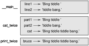
Figure 3.1
The frames are arranged in a stack that indicates which function called
which, and so on. In this example, print_twice was called by
cat_twice, and cat_twice was called by __main__, which is a
special name for the topmost frame. When you create a variable outside
of any function, it belongs to __main__.
Each parameter refers to the same value as its corresponding argument. So, part1 has the same value as line1, part2 has the same value as line2, and bruce has the same value as cat.
If an error occurs during a function call, Python prints the name of the
function, the name of the function that called it, and the name of the
function that called that, all the way back to
__main__.
For example, if you try to access cat from within
print_twice, you get a NameError:
Traceback (innermost last):
  File "test.py", line 13, in __main__
    cat_twice(line1, line2)
  File "test.py", line 5, in cat_twice
    print_twice(cat)
  File "test.py", line 9, in print_twice
    print(cat)
NameError: name 'cat' is not defined
This list of functions is called a traceback. It tells you what program file the error occurred in, and what line, and what functions were executing at the time. It also shows the line of code that caused the error.
The order of the functions in the traceback is the same as the order of the frames in the stack diagram. The function that is currently running is at the bottom.
3.10 Fruitful functions and void functions
Some of the functions we have used, such as the math functions, return
results; for lack of a better name, I call them fruitful
functions. Other functions, like print_twice, perform an
action but don’t return a value. They are called void
functions.
When you call a fruitful function, you almost always want to do something with the result; for example, you might assign it to a variable or use it as part of an expression:
x = math.cos(radians)
golden = (math.sqrt(5) + 1) / 2
When you call a function in interactive mode, Python displays the result:
>>> math.sqrt(5)
2.2360679774997898
But in a script, if you call a fruitful function all by itself, the return value is lost forever!
math.sqrt(5)
This script computes the square root of 5, but since it doesn’t store or display the result, it is not very useful.
Void functions might display something on the screen or have some other effect, but they don’t have a return value. If you assign the result to a variable, you get a special value called None.
>>> result = print_twice('Bing')
Bing
Bing
>>> print(result)
None
The value None is not the same as the string 'None'. It
is a special value that has its own type:
>>> type(None)
<class 'NoneType'>
The functions we have written so far are all void. We will start writing fruitful functions in a few chapters.
3.11 Why functions?
It may not be clear why it is worth the trouble to divide a program into functions. There are several reasons:
-
Creating a new function gives you an opportunity to name a group of statements, which makes your program easier to read and debug.
-
Functions can make a program smaller by eliminating repetitive code. Later, if you make a change, you only have to make it in one place.
-
Dividing a long program into functions allows you to debug the parts one at a time and then assemble them into a working whole.
-
Well-designed functions are often useful for many programs. Once you write and debug one, you can reuse it.
3.12 Debugging
One of the most important skills you will acquire is debugging. Although it can be frustrating, debugging is one of the most intellectually rich, challenging, and interesting parts of programming.
In some ways debugging is like detective work. You are confronted with clues and you have to infer the processes and events that led to the results you see.
Debugging is also like an experimental science. Once you have an idea about what is going wrong, you modify your program and try again. If your hypothesis was correct, you can predict the result of the modification, and you take a step closer to a working program. If your hypothesis was wrong, you have to come up with a new one. As Sherlock Holmes pointed out, “When you have eliminated the impossible, whatever remains, however improbable, must be the truth.” (A. Conan Doyle, The Sign of Four)
For some people, programming and debugging are the same thing. That is, programming is the process of gradually debugging a program until it does what you want. The idea is that you should start with a working program and make small modifications, debugging them as you go.
For example, Linux is an operating system that contains millions of lines of code, but it started out as a simple program Linus Torvalds used to explore the Intel 80386 chip. According to Larry Greenfield, “One of Linus’s earlier projects was a program that would switch between printing AAAA and BBBB. This later evolved to Linux.” (The Linux Users’ Guide Beta Version 1).
3.13 Vocabulary
- function:
- A named sequence of statements that performs some useful operation. Functions may or may not take arguments and may or may not produce a result.
- function definition:
- A statement that creates a new function, specifying its name, parameters, and the statements it contains.
- function object:
- A value created by a function definition. The name of the function is a variable that refers to a function object.
- header:
- The first line of a function definition.
- body:
- The sequence of statements inside a function definition.
- parameter:
- A name used inside a function to refer to the value passed as an argument.
- function call:
- A statement that runs a function. It consists of the function name followed by an argument list in parentheses.
- argument:
- A value provided to a function when the function is called. This value is assigned to the corresponding parameter in the function.
- local variable:
- A variable defined inside a function. A local variable can only be used inside its function.
- return value:
- The result of a function. If a function call is used as an expression, the return value is the value of the expression.
- fruitful function:
- A function that returns a value.
- void function:
- A function that always returns None.
- None:
- A special value returned by void functions.
- module:
- A file that contains a collection of related functions and other definitions.
- import statement:
- A statement that reads a module file and creates a module object.
- module object:
- A value created by an import statement that provides access to the values defined in a module.
- dot notation:
- The syntax for calling a function in another module by specifying the module name followed by a dot (period) and the function name.
- composition:
- Using an expression as part of a larger expression, or a statement as part of a larger statement.
- flow of execution:
- The order statements run in.
- stack diagram:
- A graphical representation of a stack of functions, their variables, and the values they refer to.
- frame:
- A box in a stack diagram that represents a function call. It contains the local variables and parameters of the function.
- traceback:
- A list of the functions that are executing, printed when an exception occurs.
3.14 Exercises
Write a function named right_justify that takes a string named
s as a parameter and prints the string with enough leading
spaces so that the last letter of the string is in column 70 of the
display.
>>> right_justify('monty')
                                                                 monty
Hint: Use string concatenation and repetition. Also, Python provides a
built-in function called len that returns the length of a
string, so the value of len('monty') is 5.
A function object is a value you can assign to a variable or pass as an
argument. For example, do_twice is a function that takes a function
object as an argument and calls it twice:
def do_twice(f):
    f()
    f()
Here’s an example that uses do_twice to call a function named
print_spam twice.
def print_spam():
    print('spam')

do_twice(print_spam)
-
Type this example into a script and test it.
-
Modify
do_twiceso that it takes two arguments, a function object and a value, and calls the function twice, passing the value as an argument. -
Copy the definition of
print_twicefrom earlier in this chapter to your script. -
Use the modified version of
do_twiceto callprint_twicetwice, passing'spam'as an argument. -
Define a new function called
do_fourthat takes a function object and a value and calls the function four times, passing the value as a parameter. There should be only two statements in the body of this function, not four.
Solution: http://thinkpython2.com/code/do_four.py.
Note: This exercise should be done using only the statements and other features we have learned so far.
-
Write a function that draws a grid like the following:
+ - - - - + - - - - +
|         |         |
|         |         |
|         |         |
|         |         |
+ - - - - + - - - - +
|         |         |
|         |         |
|         |         |
|         |         |
+ - - - - + - - - - +
Hint: to print more than one value on a line, you can print a comma-separated sequence of values:
print('+', '-')By default, print advances to the next line, but you can override that behavior and put a space at the end, like this:
print('+', end=' ')
print('-')
The output of these statements is
'+ -'on the same line. The output from the next print statement would begin on the next line. -
Write a function that draws a similar grid with four rows and four columns.
Solution: http://thinkpython2.com/code/grid.py. Credit: This exercise is based on an exercise in Oualline, Practical C Programming, Third Edition, O’Reilly Media, 1997.